Vectors, functions, and stacking
A vector is just an ordered list of numbers, for example, x = (88, 91, 76) is a vector in \mathbf{R}^3.
A matrix is a rectangular grid of numbers. One of the more useful properties of a matrix is that it transforms a vector into another vector. Multiplying a vector by a matrix produces a new vector, typically of a different length, whose entries are weighted sums of the original entries.
A function f takes an input and produces an output, y = f(x).
Neural networks are built by chaining functions together; the output of one becomes the input of the next. If you have three functions f_1, f_2, f_3, chaining them means computing
We call this function composition, and every neural network, no matter how exotic, is fundamentally a long composition like this. Each f_i is called a layer. Modern language models chain together anywhere from a few dozen to a few hundred layers. The input x_0 starts as a representation of some text; each layer nudges that representation a little, and the final layer’s output is used to make a prediction (such as “what word comes next”).
Each f_i function has some internal numbers (weights, written as W_i) that are adjusted during training so the whole composition produces better results.
These weights are adjusted via the derivative of the output with respect to each weight, and computing that derivative for an early layer requires the chain rule, differentiating a composition of functions.
Chain rule
If
y = f_3(f_2(f_1(x))), then\dfrac{dy}{dx} = f_3'(\cdot) \cdot f_2'(\cdot) \cdot f_1'(\cdot). The derivative of a composition is the product of the individual derivatives.
Why depth is hard
Suppose you stack L layers instead of 3. Training uses a procedure called backpropagation, which is really just the chain rule applied over and over, from the last layer back to the first. To figure out how much the very first layer’s weights should change, you need the derivative of the final output with respect to the first layer’s input.
By the chain rule, that derivative is a product of L terms, one per layer:
Suppose each individual derivative f_i happens to be, on average, a bit less than 1; for our example, we’ll say 0.9. What happens to the product as L grows?
By 200 layers, the gradient reaching the first layer is ten orders of magnitude smaller than the gradient at the last layer. In the real world, we deal with finite precision floating-point arithmetic, and this is indistinguishable from zero. The first layer effectively stops learning, as its weight updates are microscopic no matter how wrong its output is.
This is the famous vanishing gradient problem.
The same failure happens in the other direction, when the average derivative is a bit larger than 1, causing the product to blow up instead; the exploding gradient problem. Either way, depth alone destabilizes training, purely as a consequence of multiplying many numbers together.
In a real network, this collapse happens not for a scalar, but for a vector, so the derivative of each f_i is really a Jacobian matrix (a grid of partial derivatives) rather than a single number. In that context “small” means something like “shrinks vectors on average”, or formally, its spectral norm (the largest factor by which the matrix can stretch a vector) is less than 1.
But the end result looks the same: composing many maps that each shrink (or grow) space by roughly the same factor shrinks (or grows) it exponentially in depth.
Residual Connections
In 2015, Kaiming He and coauthors at Microsoft Research proposed residual connections. Instead of a layer replacing its input, it adds a correction to it.
Compare this to the plain version, x_{l+1} = F(x_l, W_l). The difference may look small, just one extra addition, but it has a big impact. F is now called the residual function; it doesn’t have to reconstruct the entire next representation from scratch, it only has to compute a correction to add on top of what’s already there.
If the best thing a layer can do is nothing at all, it can learn to make F output approximately zero, and the identity simply passes through.
When we unroll this recurrence across several layers, something clean happens. Starting from layer l and applying the rule repeatedly up to layer L:
We get a telescoping sum. The deeper representation x_L is just the shallow representation x_l plus a running total of corrections. Importantly, x_l appears undiminished; it isn’t multiplied by anything. Differentiate this expression and the chain-rule product from the previous section gets an extra additive term at every layer:
where I is the identity map. Composing many of these no longer multiplies L numbers that are each a bit less than one; it multiplies L terms that are each close to one, because they’re “1 plus something,” and that something is typically kept small by how the layer is initialized and normalized. The gradient signal has, in He et al.’s words, an unimpeded shortcut through which information can flow from the last layer to the first layer through pure addition.
Hyper-connections
In 2024, a team at ByteDance’s Seed Foundation Model group asked an interesting question. If one identity shortcut is so great, is having several of them better?
The residual connection carries exactly one “lane” of information forward, x_l, a single vector of dimension C. Zhu et al.’s Hyper-Connections (HC) widen that single lane into n parallel lanes, an n-stream residual, and replace the fixed “add” and “read” operations with learnable matrices that control how information moves between the lanes and the layer.
Concretely, instead of a vector x_l \in \mathbf{R}^{1\times C}, HC carries a small matrix \mathbf{x}_l \in \mathbf{R}^{n\times C}; literally n stacked copies of the residual stream, each of width C. Three learnable maps govern what happens at each layer:
H^{pre}_l \in \mathbf{R}^{1\times n}, a read map. It takes a weighted combination of thenlanes and collapses them into the singleC-dimensional vector that the layer function actually operates on.H^{post}_l \in \mathbf{R}^{1\times n}, a write map. It takes the layer’s single output vector and scatters it back out across thenlanes.H^{res}_l \in \mathbf{R}^{n\times n}, a mixing map. It lets thenlanes exchange information directly with one another, without passing through the layer function.
Put together, one layer of Hyper-Connections computes:
What does this buy you? There are two aspects that the HC paper emphasizes.
First, H^{res}_l can learn to weight some lanes more heavily than others depending on what’s useful at that depth. The network can dynamically adjust how strongly information from different points in the stack influences the other lanes, rather than relying on the fixed behavior of a plain residual connection.
Second, because H^{res}_l is not required to be close to the identity, it can act like a soft permutation, effectively letting the network rearrange which lane’s information dominates at which depth.
We can describe the residual connection as a Hyper-Connection with n=1, as H^{res}_l collapses to the scalar 1 and the rest of the equation reduces to x_{l+1} = x_l + F(x_l, W_l).
An Unconstrained Matrix
Recall the telescoping sum for plain residual connections, unrolled across depth, x_l passes through untouched, multiplied by nothing. Now do the same unrolling for Hyper-Connections.
Because the “skip” term is now H^{res}_l\,\mathbf{x}_l rather than \mathbf{x}_l itself, propagating a signal from a shallow layer l to a deeper layer L multiplies it by a whole chain of matrices.
That leading product, \prod_{i=1}^{L-l} H^{res}_{L-i}, is exactly the same kind of object that caused the vanishing/exploding gradient problem before. A long chain of matrix multiplications, except now it’s sitting where the previously well-behaved identity matrix used to be.
H^{res}_l is unconstrained; it’s just whatever a neural network happens to learn with no guarantee that multiplying sixty of them in a row does anything reasonable to a vector’s scale.
When the DeepSeek team trained large (27-billion-parameter) models with Hyper-Connections, they measured how much a composite chain of H^{res} matrices could amplify a signal. They call the largest row sum of the accumulated product the Amax Gain Magnitude. For a single layer, this stayed close to a sensible range. Accumulated across greater depths, it reached peaks in the thousands.
A signal—or, running backward, a gradient—passing through the residual stream could be amplified a thousand-fold purely by the residual path, before the layer functions F even entered the computation. In their training runs this showed up as a big loss spike partway through training, correlated with a burst in gradient norm.
Furthermore, there’s another, more mundane problem. Widening the residual stream from one lane to n lanes means every read and write to that stream costs roughly n times as much memory traffic. On modern accelerators, moving data is often more expensive than computing it.
The paper published by the DeepSeek team solved both of these issues, and in a surprisingly simple way.
A crash course on manifolds
The word “manifold” sounds intimidating mostly because of how it’s usually introduced. The idea itself is simple: it is a shape that looks flat if you’re standing close enough to it, even if it’s curved overall.
A classic example is the Earth. Stand in a field and the ground looks flat, ordinary two-dimensional flat space, the kind you learned coordinate geometry on. Zoom out to the scale of continents and it’s obviously a curved sphere.
A manifold is exactly this idea made more precise; a space that locally resembles ordinary flat (Euclidean) space around every point, even though its global shape can be curved, closed, or otherwise exotic.1
A circle is a one-dimensional manifold; zoom in anywhere on it and it looks like a straight line segment. A sphere’s surface is a two-dimensional manifold. A figure-eight is not a manifold, because at the crossing point, no amount of zooming in makes it look like a simple flat line; two strands cross there, and no local view is just “flat”.
Why do we care about this? Consider a recurring pattern we’ve seen in neural-network optimization up till now. We often want to adjust a quantity, such as a vector or matrix, while requiring it to always satisfy some structural property. A unit vector must always have length 1. A rotation matrix must always preserve distances and orientation. A probability distribution’s entries must always be non-negative and sum to 1.
In every one of these cases, the “legal” values don’t form all of \mathbf{R}^n. They form a curved, lower-dimensional subset sitting inside it. If that subset is well-behaved (locally flat, in the manifold sense), there’s an elegant recipe for optimizing over it. We take an ordinary step in the surrounding flat space, not considering the real shape because we’re zoomed in so far, then project back onto the subset, like “snapping” back onto the allowed shape.
This is the core of an entire field called Riemannian optimization, or manifold optimization.
A little insert for those who care
The set of doubly-stochastic matrices we’re about to meet, the actual “manifold” in Manifold-Constrained Hyper-Connections, is technically a polytope, a convex shape with flat faces and sharp corners and edges, defined by a finite list of linear equalities and inequalities. It is not a manifold in the strict textbook sense of the word at its corners and edges, because near a corner the shape doesn’t look locally flat in every direction, it looks like a wedge. Only the interior is a smooth manifold. In practice, the machine-learning community uses “manifold” a good deal more loosely than differential geometers do, meaning a constrained, structured space you can define a sensible projection onto, whether or not every point of it is technically a smooth-manifold point.
Doubly-stochastic matrices and the Birkhoff polytope
A square matrix H \in \mathbf{R}^{n\times n} is called doubly stochastic if it satisfies three conditions:
In English, every entry is non-negative, every row sums to 1, and every column sums to 1 (\mathbf{1}_n is just the all-ones vector; multiplying by it computes a sum). If you drop the column condition and keep only “non-negative, rows sum to 1,” you get an ordinary stochastic matrix, also known as the transition matrix of a Markov chain, or a matrix whose rows are each a probability distribution. Demanding both rows and columns sum to 1 is a much stronger and more symmetric condition.
The simplest doubly-stochastic matrices are permutation matrices, square 0/1 matrices with exactly 1 in every row and every column; everything else is 0. A permutation matrix doesn’t blend anything, it just reorders coordinates. For n=3 there are exactly 3! = 6 of them, one for each way of shuffling three items:
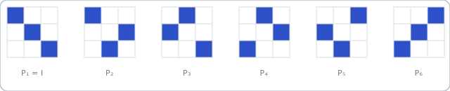
Permutation matrices are the extreme, “pure” cases. But they’re not the only doubly-stochastic matrices; you can also average them together. If P_1, \dots, P_6 are the six permutation matrices above and \lambda_1, \dots, \lambda_6 are non-negative weights summing to 1, then \sum_i \lambda_i P_i is also doubly-stochastic.
A remarkable theorem, proven by Garrett Birkhoff in 1946, though equivalent statements go back to Kőnig and Steinitz decades earlier2, says the converse is also true.
Birkhoff-von Neumann theorem
Every
n\times ndoubly-stochastic matrix can be written as a convex combination (a weighted average with non-negative weights summing to 1) ofn\times npermutation matrices. Equivalently, the set of all doubly-stochastic matrices is exactly the convex hull of the permutation matrices; no more, no less.
There are two properties of this polytope that become useful to the use case described in this piece.
A doubly-stochastic matrix cannot stretch a vector
The spectral norm \|H\|_2 of a matrix measures the largest factor by which it can stretch any vector’s length; \|Hv\| \leq \|H\|_2\,\|v\| for every v. A permutation matrix simply reorders a vector’s entries, which cannot change its length at all; so \|P\|_2 = 1 exactly, for any permutation matrix P.
Now take a doubly-stochastic H = \sum_i \lambda_i P_i. The spectral norm is itself a norm on the space of matrices, so it obeys the triangle inequality:
So every doubly-stochastic matrix has spectral norm at most 1. It can shrink or preserve a vector’s length, but it can never amplify it. If we could somehow apply this idea to the residual stream we discussed before, it would stop our signal from exploding.
The product of two doubly-stochastic matrices is doubly-stochastic
Take A,B both doubly-stochastic. Their product AB is entrywise non-negative, since it’s built from sums of products of non-negative numbers.
For the row sums, (AB)\mathbf{1}_n = A(B\mathbf{1}_n) = A\mathbf{1}_n = \mathbf{1}_n.
For the column sums, by the same argument on the transpose, \mathbf{1}_n^\top(AB) = (\mathbf{1}_n^\top A)B = \mathbf{1}_n^\top B = \mathbf{1}_n^\top.
So AB is again doubly-stochastic. We call this closure under multiplication.
Put these two facts together and you get exactly the guarantee we were missing before. If every H^{res}_l is doubly-stochastic, then by the second property, any product of them, \prod_i H^{res}_{L-i}, is also doubly-stochastic, no matter how deep the network is!
And by the first property, that product has spectral norm at most 1, at every depth, not just on average. The composite mapping can never amplify a signal, regardless of how many layers you compose. We have basically restored the identity mapping property we had before, not that H^{res}_l equals the identity matrix exactly (that would prevent the streams from mixing), but that it’s drawn from a family of matrices that is provably non-expansive under many repeated compositions.
Projecting onto the polytope
Knowing the target shape we want is only half the problem! We also need a cheap, differentiable way to push an arbitrary matrix, whatever a neural network happens to output, onto it, at every layer, on every forward pass, for every token.
Funny enough, the algorithm ends up being embarrassingly simple, and it predates deep learning by decades, with versions of it appearing in the 1940s survey statistics under the name “iterative proportional fitting”. It was analyzed rigorously for matrices by Richard Sinkhorn in 1964 and jointly with Paul Knopp in 1967.3
Start with any matrix that has only positive entries. Then repeat two steps:
- Divide every row by its own sum, so all rows sum to exactly 1.
- Divide every column by its own sum, so all columns sum to exactly 1.
The catch, obviously, is that step 2 can undo step 1’s row sums a little bit; dividing a column by its sum changes every entry in that column, including the row totals we just fixed.
But there’s a nice way around this. Each round of doing both steps damages the previous step’s work by a shrinking amount. Sinkhorn and Knopp proved that for any square matrix with strictly positive entries, this alternation converges, and does so linearly, meaning the error shrinks by roughly a constant factor every round.
The result of the convergence is a doubly-stochastic matrix. A handful of iterations is normally enough to get within floating-point precision of the exact answer.4
For us to apply this idea inside a neural network layer, two adaptations are needed. First, the network doesn’t naturally produce positive numbers; its raw output for H^{res}_l can be any real number. So the first step is to exponentiate every entry, guaranteeing positivity while keeping the whole operation smooth and differentiable.
Second, since the algorithm only reaches the exact answer in the limit, a practical implementation fixes a finite iteration count. The DeepSeek team settled on t_{\max}=20, enough to be indistinguishable from exact in ordinary floating-point precision. Concretely, writing \tilde{H}^{res}_l for the network’s raw, unconstrained output at layer l:
where T_r and T_c denote row- and column-normalization, respectively. The output H^{res}_l is, to numerical precision, a doubly-stochastic matrix, a point inside the Birkhoff polytope.
Another insert for those who care
If this iteration looks familiar from a different corner of machine learning, that’s because it is. The same alternating-normalization idea became a commonly used tool in computational optimal transport after Marco Cuturi’s 2013 paper Sinkhorn Distances showed that adding an entropy penalty to the classic transportation problem turns its solution into exactly this kind of iterative matrix scaling.5
Manifold-Constrained Hyper-Connections
Finally, we can discuss Manifold-Constrained Hyper-Connections (mHC). mHC is what you get when you take Hyper-Connections and force H^{res}_l to always live on the Birkhoff polytope.
Formally, define the projection of the residual-mixing map onto the manifold of doubly-stochastic matrices:
Substituting this constrained matrix into the Hyper-Connections layer equation gives the full mHC:
One more small piece, H^{pre}_l and H^{post}_l, the read and write maps, are also constrained, though more gently. Rather than forcing them onto a polytope, the paper simply forces every entry to be non-negative, using a sigmoid function (\sigma). This clamps the entries of H^{pre}_l into the range (0,1) and those of H^{post}_l into (0,2).
The reasoning behind this choice is similar. If H^{pre}_l were allowed both positive and negative entries, the network could, in principle, learn a read map that looks large in magnitude, suggesting an active and expressive mixing, while its positive and negative parts nearly cancel out, contributing almost nothing and hiding that fact from any weight-magnitude diagnostic.
Forcing non-negativity closes off that particular failure mode, as every lane’s contribution adds, rather than potentially fighting against another lane. It’s a milder constraint than the full doubly-stochastic one, H^{pre}_l and H^{post}_l aren’t required to sum to any particular total, but I think it’s philosophically the same idea.
The raw, pre-projection values themselves, \widetilde{H}^{pre}_l, \widetilde{H}^{post}_l, \widetilde{H}^{res}_l, are computed from the current hidden state in two parts, a static component (a learned bias, same for every token) plus a dynamic component (a small linear readout of the current, normalized hidden state, scaled by a learnable gate):
Nothing there is new; RMSNorm is a well-known normalization method.
The bigger picture
Researchers often distinguish micro-designs (what a single block computes, attention, convolutions, feed-forward) from macro-design (the topology connecting blocks together). The last decade of micro-design progress is more well-known, with advancements such as attention, Mixture-of-Experts routing, and so on.
Macro-design has its own, less well-known, history. After the original residual connection, DenseNet connected every layer directly to every later layer;6 FractalNet built networks out of self-similar branching sub-structures instead of a single chain;7 Highway Networks, which slightly predate ResNet, used a learned gate to blend a layer’s output with its input;8 Deep Layer Aggregation proposed recursively merging features across both depth and resolution.9 More recently, DenseFormer re-weighted contributions from all previous layers at every step,10 MUDDFormer built dynamic, content-dependent dense connections across a transformer stack,11 and Residual Matrix Transformers replaced the residual vector entirely with an outer-product memory matrix.12
All of these approachs have some trade-off between, more connectivity buys more expressiveness, but identity-mapping allows deep training to be tractable. The mHC paper gives us a way to describe the stability of very deep networks as a geometric property of the space a matrix is allowed to live in.
The solution described by mHC can be generalized to settings well beyond the transformer blocks the original paper tested. Within a few months of the paper releasing, researchers had already adapted the same doubly-stochastic constraint to graph neural networks, where it slows the over-smoothing problem from decaying exponentially in depth to decaying exponentially in depth divided by the stream width.13 The approach has also been applied to state-space sequence models in the Mabma family.14
Another line of follow-up work asks whether the Sinkhorn-Knopp approximation, which only reaches the exact polytope in the limit of infinitely many iterations, can be replaced with something more exact. One proposal restricts H^{res}_l to literal convex combinations of a small set of permutation matrices. This guarantees exactness at the cost of a combinatorial blow-up in how many permutations you need to track. A follow-up called TBP-mHC instead generalizes to a broader family called transporation polytopes to recover more expressive power, while a concurrent approach nicknamed KromHC uses Kronecker-product structure to keep the parameter count down by restricting to a smaller, structured slice of the Brikhoff polytope.15
The apper’s own conclusion gestures at where this plausibly goes next: doubly-stochastic matrices are just one choice of manifold, chosen because it maps cleanly onto “conservation of signal energy.” Other constrained sets encode other properties a network designer might want; matrices that preserve angles as well as lengths (orthogonal matrices, forming what’s called the Stiefel manifold), or matrices with a fixed, bounded rank. All of these are already-studied objects in the Riemannian-optimization literature we discussed before, and none of them are specific to language models.
If mHC’s core idea holds up, the question that will be the most interesting in the long-run won’t really be about hyper-connections, but about which other pieces of a deep network’s plumbing turns out to be, in disguise, constrained-optimization problems.